1. Definition
"Hyperbola - The set of all points such that the difference in the distance from two points is a constant." (Crystal Kirch)
2. Descriptions
 |
| https://blogger.googleusercontent.com/img/b/R29vZ2xl/AVvXsEj0qtmzjxnQMmKSnAlrxQP1qAjNVV0kPZ_XFMTLWIKxA1PqrclwGhZtpy7P0o_JjIKT6uhywOllyV_gtKLT9T84mOjKEgxM1EHRRrQPxo7YcmwBF-Jh-fmEkCb0ZJOmo6y_4jx5nLIMLzO7/s400/hyperbola.jpg |
 |
| http://www.mathwarehouse.com/hyperbola/images/compare-hyperbola-graphs.gif |
http://www.youtube.com/watch?v=dn1o6lpu_Sk
Key Parts
The
center is written as an ordered pair (x,y), and it marks the midpoint of
the entire graph. It can be identified algebraically by identifying
the "h" and "k" values from the equation. Note that "x" is always
partnered with "h", and "y" is always partnered with "k". It can be
identified graphically as the point directly in between the drawings of
the two asymptotes. The transverse axis is written as an equation. It
connects the asymptotes and contains the two vertices; it is
perpendicular to the conjugate axis. If “x” comes before “y”, then the axis
is written as “y= ”. Vice versa, if “y” comes before “x”, then the axis is
written as “x=”. The axis usually appears as a solid line connecting the two
graphs of the asymptotes. The conjugate axis is written as an equation;
it runs in between the asymptotes, contains the two co-vertices, and is
perpendicular to the transverse axis. If “x” comes after “y”, then the axis
is written as “x= ”. Vice versa, if “y” comes after “x”, then the axis is
written as “y=”. The conjugate axis is usually drawn as a dashed line that runs in between but never touches the asymptotes.
The vertices are written as ordered pairs. They determine the starting point of each asymptote and lie along the transverse axis. The “x” value of the vertices can be found by moving “a” units from the center along the transverse axis. The center and the vertices have a common “y” value”. The vertices can be found at the point when the asymptotes touch the transverse axis. The co-vertices are written as ordered pairs and they lie along the conjugate axis. The co-vertices and the center share the same “x” value. The “y” value of the vertices can be found by moving “b” units from the center along the conjugate axis. The co-vertices can be found at the ends of the conjugate axis that runs between the two asymptotes. The foci are written as ordered pairs and are located in between each of the asymptotes and determine their width. The further the foci are from the asymptote, the thinner the asymptote becomes and the higher the eccentricity (vice versa). The “x” values of the foci can be found by moving “c” units away from the center along the transverse axis. The foci and the center share the same “y” value. The foci are identified as the points within the opening of the vertices that are “c” units away from the center.
The vertices are written as ordered pairs. They determine the starting point of each asymptote and lie along the transverse axis. The “x” value of the vertices can be found by moving “a” units from the center along the transverse axis. The center and the vertices have a common “y” value”. The vertices can be found at the point when the asymptotes touch the transverse axis. The co-vertices are written as ordered pairs and they lie along the conjugate axis. The co-vertices and the center share the same “x” value. The “y” value of the vertices can be found by moving “b” units from the center along the conjugate axis. The co-vertices can be found at the ends of the conjugate axis that runs between the two asymptotes. The foci are written as ordered pairs and are located in between each of the asymptotes and determine their width. The further the foci are from the asymptote, the thinner the asymptote becomes and the higher the eccentricity (vice versa). The “x” values of the foci can be found by moving “c” units away from the center along the transverse axis. The foci and the center share the same “y” value. The foci are identified as the points within the opening of the vertices that are “c” units away from the center.
The value of "a" is written as a numerical value that represents the distance between one vertex and the center. In a standard form equation, the
squared value of “a” can be found underneath the first fraction. Graphically, the value can be identified by counting the number of units between the center and a vertex. "b" is also written as a numerical value that represents the distance between one co-vertex and the center. In
a standard form equation, the
squared value of “b” can be found underneath the second fraction. It can
be identified graphically by counting the number of units between one
co-vertex and the center. The value of "c" is written as a numerical value and it measures the distance between one foci and the center. After obtaining the values of “a” and “b” from the
equation, you can identify “c” plugging in the
appropriate numbers into: a^2 + b^2 = c^2. Graphically, it can be found
by counting the number of units between the center and one foci.
Eccentricity is written as a numerical value. It measures how much a conic section isn't circular. It can be found algebraically by dividing the value of "c" by "a". Because the graph depicts a hyperbola, we know that the eccentricity is greater than one. The asymptotes are written as equations; they start at the vertices and extend rightward and leftward away from the center. If “x” comes before “y” in the equation, the asymptote open left and right; vice versa, the asymptotes open up and down. The asymptotes can be identified by finding two points on the line, or by finding the center and the slope using b/a for horizontal graphs, and a/b for vertical graphs. The standard form is the typical way of writing the equation of a hyperbola. You can find it by completing the square and using the information provided to fill in all the needed parts. You can identify it graphically by following the said steps to complete the necessary parts. Set everything equal to "1" to complete the equation. To learn more about how to graph hyperbolas from standard form, watch the above video here!
Eccentricity is written as a numerical value. It measures how much a conic section isn't circular. It can be found algebraically by dividing the value of "c" by "a". Because the graph depicts a hyperbola, we know that the eccentricity is greater than one. The asymptotes are written as equations; they start at the vertices and extend rightward and leftward away from the center. If “x” comes before “y” in the equation, the asymptote open left and right; vice versa, the asymptotes open up and down. The asymptotes can be identified by finding two points on the line, or by finding the center and the slope using b/a for horizontal graphs, and a/b for vertical graphs. The standard form is the typical way of writing the equation of a hyperbola. You can find it by completing the square and using the information provided to fill in all the needed parts. You can identify it graphically by following the said steps to complete the necessary parts. Set everything equal to "1" to complete the equation. To learn more about how to graph hyperbolas from standard form, watch the above video here!
3. Real World Application
 |
| http://www.a-levelphysicstutor.com/images/optics/lnss-ccv-ray02.jpg |
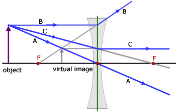
Hyperbolas, which are found within several variations of math and science, can be applied to everyday life! One of the most common, and possibly the most overlooked example is the use of hyperbolas in glasses and telescopes. Of the two types of lenses that are manufactured, the one that applies the properties of hyperbolas is known as a concave lens. This lens helps people to see objects from greater distances.
Similar to our graphs of hyperbolas, the lens has two curves that cave inwards in opposite directions. Likewise, there is a focus point within each of the curves. Concave lenses diffracts, or changes the direction of light waves. As a result, a virtual image of what is actually seen appears on the opposite side of the focal point, nearer the lens. To learn more about concave lenses and their application of hyperbolas, click here.
4. Works Cited
- http://www.lessonpaths.com/learn/i/unit-m-conic-section-applets/hyperbola-from-the-definition-geogebra-dynamic-worksheet
- https://blogger.googleusercontent.com/img/b/R29vZ2xl/AVvXsEj0qtmzjxnQMmKSnAlrxQP1qAjNVV0kPZ_XFMTLWIKxA1PqrclwGhZtpy7P0o_JjIKT6uhywOllyV_gtKLT9T84mOjKEgxM1EHRRrQPxo7YcmwBF-Jh-fmEkCb0ZJOmo6y_4jx5nLIMLzO7/s400/hyperbola.jpg
- http://www.mathwarehouse.com/hyperbola/images/compare-hyperbola-graphs.gif
- http://www.a-levelphysicstutor.com/images/optics/lnss-ccv-ray02.jpg
- http://www.youtube.com/watch?v=dn1o6lpu_Sk
- https://www.khanacademy.org/science/physics/waves-and-optics/v/concave-lenses
To learn more about conic sections, visit Crystal Kirch's blog here!
No comments:
Post a Comment